My previous blog discussed some historical papers related to the intensity interferometer and its connection to quantum optics. Here, I explain the basic physics of an intensity interferometer.
In the context of spatial coherence, the coherence theory expresses the degree of spatial coherence as,
with \( U_i(t) \) representing the fields of sources \( i = 1 \) and \( 2 \).
An intensity interferometer measures the intensity correlation function between such sources. If \( I_1(t) \) is the intensity of source 1 and \( I_2(t) \) is the intensity of source 2, then the intensity correlation function is given by:
If one ignores the background (the first term in the sum of the above equation) and considers only the fluctuations in the signal (the second term), then the term of relevance will be:
The signal in the intensity interferometer is thus proportional to \( \left| \gamma_{12} \right|^2 \).
A conventional interferometer measures a signal that is proportional to \( \left| \gamma_{12} \right| \), which includes the amplitude and phase, whereas an intensity interferometer measures a signal proportional to \( \left| \gamma_{12} \right|^2 \), which is not sensitive to the phase.
Intensity interferometers have certain advantages compared to conventional interferometers (such as the Michelson interferometer). Below is a partial list:
Intensity measurements (unlike amplitude or phase) can be done directly using optoelectronic instruments.
They do not require precise, sub-wavelength optical alignment, unlike amplitude- or wavefront-dividing interferometers.
They can be used with two detectors that are placed far apart, thereby improving the spatial resolution of the measurement (relevant in astronomy).
A constraint of an intensity interferometer is that the intensity of the participating source should be bright.
There is an important connection between quantum optics and radio astronomy. Hanbury Brown and Twiss in the 1950s devised the intensity interferometer.
Particularly, they were interested in measuring the ‘diameter of discrete radio sources’. The title of their seminal paper reads “A new type of interferometer for use in radio astronomy”. As the authors claimed in their paper: “The principle of the instrument is based upon the correlation between the rectified outputs of two independent receivers at each end of a baseline, and it is shown that the cross-correlation coefficient between these outputs is proportional to the square of the amplitude of the Fourier transform of the intensity distribution across the source.”(Brown and Twiss, 1954)
First, they tested their technique in a laboratory situation and followed it up with a measurement of the diameter of Sirius. Their technique was a game-changer in measuring the diameter of bright stars.
As the intensity interferometers were being developed, the laser was realized in the early 1960s. Unlike conventional light sources, laser light is coherent, and this brings in unique features that can be used to understand the nature of light. In the context of laser optics, intensity interferometers had immediate utility in studying coherence through correlation measurement. It was logical to combine lasers with intensity interferometers and study the correlation. This combination is what led to the discovery of some fascinating aspects of quantum properties of light, including anti-bunching.
If the book by Born and Wolf is considered a classic on the electromagnetic theory of light, the quantum extrapolation is the book by Leonard Mandel and Emil Wolf titled Optical Coherence and Quantum Optics.
This book discusses the interface of statistical optics, optical coherence, and quantum optics. The core argument of the book starts with probability theory and its connection to fluctuations of light and builds optical coherence, polarization, and eventually quantum optical effects of light. It is a well-written treatise on light with a flavor of experiments (Mandel did some pioneering experiments in quantum optics) and theoretical explanation (a hallmark of Wolf).
In the preface of the book, they bring together the importance of intensity interferometers and the discovery of lasers and explain how and why it led to a deeper understanding of quantum optics:
“Prior to the development of the first lasers in the 1960s, optical coherence was not a subject with which many scientists had much acquaintance, even though early contributions to the field were made by several distinguished physicists, including Max von Laue, Erwin Schrodinger and Frits Zernike. However, the situation changed once it was realized that the remarkable properties of laser light depended on its coherence. An earlier development that also triggered interest in optical coherence was a series of important experiments by Hanbury Brown and Twiss in the 1950s, showing that correlations between the fluctuations of mutually coherent beams of thermal light could be measured by photoelectric correlation and two-photon coincidence counting experiments. The interpretation of these experiments was, however, surrounded by controversy, which emphasized the need for understanding the coherence properties of light and their effect on the interaction between light and matter.” (Mandel and Wolf, 1995, p. 1)
This further led to a series of studies on light-matter interaction from a coherence perspective, and included analysis of the fluctuation of light by understanding the randomness and the associated statistics of the fluctuations. Mandel, Wolf, Glauber, E.C.G. Surdarshan and many others across the world laid the foundation and connection between optical coherence and quantum optics. What started as a technical development in radio astronomy turned out to be a vital tool in quantum optics.
Brown, R. Hanbury, and R. Q. Twiss. ‘LXXIV. A New Type of Interferometer for Use in Radio Astronomy’. Philosophical Magazine 45, no. 366 (1954): 663–82. https://doi.org/10.1080/14786440708520475.
Brown, R. Hanbury, and R. Q. Twiss. ‘Correlation between Photons in Two Coherent Beams of Light’. Nature 177, no. 4497 (1956): 27–29. https://doi.org/10.1038/177027a0.
Hanbury Brown, R., and R. Q. Twiss. ‘A Test of a New Type of Stellar Interferometer on Sirius’. Nature 178, no. 4541 (1956): 1046–48. https://doi.org/10.1038/1781046a0.
If you need to admire complex analysis for its elegance and visual utility, try quantum optics. Specifically, the description of quantum states. Thanks to creation and annihilation operators, the position and momentum states of a quantum optical field can be represented as quadratures. These entities can now be represented on the orthogonal axes of a complex plane. The representation of Argand diagrams starting with a classical electromagnetic field and then extrapolating them to quantum theory is a tribute to its geometrical representation. The fact that two axes can be utilized to represent real and imaginary parts of the defined state is itself an interesting thing. By certain operations within the plane, one can realize the vacuum state, the coherent state, and the squeezed state of quantum optics.
The Vacuum Spread – One of the major consequences of quantum theory, and especially the second quantization, is the realization of the vacuum states. Even when there are zero photons, there is a residual energy in the system that manifests as vacuum states. How to define the presence or absence of a photon is a different proposition because vacuum states are also associated with something called virtual photons. That needs a separate discussion. Anyway, in a complex plane of quadrature, a vacuum state is represented by a circular blob and not a point (see fig. 1). It is the spread of the blob that indicates the uncertainty. In a way, it is an elegant representation of the uncertainty principle itself because the spread in the plane indicates the error in its measurement. Importantly, it emphasizes the point that no matter how low the energy of the system is, there is an inherent uncertainty in the quadrature of the field. This also forms the fundamental difference between a classical and a quantum state. The measurement of the vacuum fluctuation is a challenging task, but one of the most prevalent consequences of vacuum fluctuation is the oblivious spontaneous emission. If one looks at the emission process in terms of stimulated and spontaneous pathways, then the logical consequence of the vacuum state becomes evident in some literature on quantum optics. Spontaneous emission is also defined as stimulated emission triggered by vacuum state fluctuations. It is an interesting viewpoint and helps us to create a picture of the emission process vis-à-vis the stimulated emission.
Figure 1. Vacuum state representation. Note that their centre is at the origin and has a finite spread across all the quadrants. Figure adapted from ref. 2.
Another manifestation of the vacuum state is the Casimir effect, where an attractive force is induced as you bring two parallel plates close to each other. The distance being of the order of the wavelength or below this triggers a fascinating phenomenon which has deep implications not only in understanding the fundamentals of quantum optics and electrodynamics, but also in the design and development of quantum nanomechanical devices.
A shift in the plane – Coherent states are also described as displaced vacuum states, and this displacement is evident in the Argand diagrams. The quadrature can now help us visualize the uncertainty in the phase and the number of photons in the optical field. One of the logical consequences of the coherent state is the number-phase uncertainty. This gets clear if one observes the spread in the angle of the vector and the radius of the blob represented (see Fig. 2). Notice that the blob still exists. The only difference is that the location of the blob has shifted. The consequence of this spread has a deeper connection to the uncertainty in the average number of photons and the phase of the optical field. The connection to the number of photons is through the mod alpha, which essentially represents the square root of the average number of photons. Taken together, the blob in the Argand diagram represents the number-phase uncertainty.
Figure 2. Coherent state representation. Note that their centre is displaced. Figure adapted from ref. 2.
Lasers are the prototypical examples of coherent states. The fact that they obey Poissonian statistics is the direct consequence of the variance in the photon number, which is equivalent to the square root of the average number of photons. This means one can use photon statistics to discriminate between sources that are sub-Poissonian, Poissonian, or super-Poissonian in nature. The super-Poissonian case is the thermal light, and the sub-Poissonian state represents photon states whose number can reach up to 1 or 0. The coherent states sit in the middle, obeying the Poissonian statistics.
Everything has a cost – Once you have a circle with a defined area, it will be interesting to ask: Can you ‘squeeze’ this circle without changing its area? The answer is yes, and that is what manifests as a squeezed state. In this special state, one can squeeze the blob along one of the axes at the cost of a spread in the orthogonal direction. This converts the circle into an ellipse (see Fig. 3).
Figure 3. Squeezed State. Note the circle has been squeezed into an ellipse. Figure adapted from ref. 2.
Note that the area must be conserved, which means that the uncertainty principle still holds good; just that the reduction in the uncertainty along one axis is compensated by the increment in another. This geometrical trick has a deep connection to the behaviour of an optical field. If one squeezes the axis along the average number of photons, it means that you are able to create an amplitude-squeezed state. This means the uncertainty in the counting of photons in that state has reduced, albeit at the cost of the uncertainty in the measurement of phase. Similarly, if one squeezes the blob along the axis of the phase, then we end up with a lowering of the uncertainty for the optical phase. Of course, this comes at the cost of counting of number of photons. I should mention that the concept of optical phase itself is not clearly defined in quantum optics. This is because an ill-defined phase can have a value of 2π, which creates the problem. An interesting application of the phase-squeezed quantum states is in interferometric measurements. By reducing the uncertainty in the phase, one can create highly accurate measurements of phase shifts. So much so that this can have direct implications on high-precision measurements, including gravitational wave detection. The anticipation is also that such tiny shifts can be helpful in observing feeble fluctuations in macroscopic quantum systems.
Pictures can lead to more than 1,000 words. And if you add them to a quantum optical description, as in the case of the states that I have defined, they create a quantum tapestry. Perhaps this is the beauty of physics, where there is a coherence between mathematical language, geometrical representation, and physical reality. Feynman semi-jokingly may have said, “Nobody understands quantum mechanics,” but he forgot to add that there is great joy in the process of understanding through mathematical pictures. After all, he knew the power of diagrams.
References:
Ficek, Zbigniew, and Mohamed Ridza Wahiddin. Quantum Optics for Beginners. 1st edition. Jenny Stanford Publishing, 2014.
Fox, Mark. Quantum Optics: An Introduction. Oxford Master Series in Physics 15. Oxford University Press, 2006.
Gerry, Christopher C., and Peter L. Knight. Introductory Quantum Optics. Cambridge, United Kingdom ; New York, NY, 2024.
Saleh, B. E. A., and M. C. Teich. Fundamentals of Photonics. 2nd edition. Wiley India Pvt Ltd, 2012.
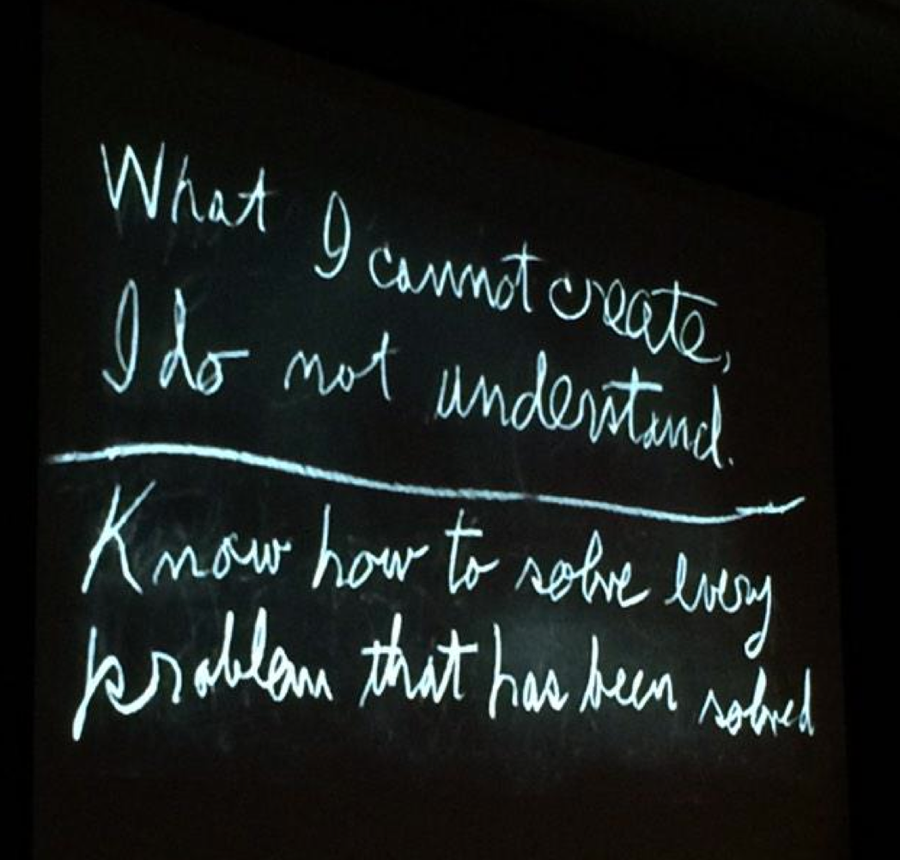
The first of these quotes by Feynman is a guiding principle for anyone who wants to learn. The second quote is an idealistic one, but a good approach to becoming a ‘problem-solving’ researcher. Feynman was a master of this approach.
From a philosophy of science perspective, researchers can be both ‘problem creators’ and ‘problem solvers’. The latter ones are usually famous.
Michael Nielsen, a pioneer of quantum computing and champion of open science movement, has an essay titled: Principles of Effective Research, in which he explicitly identifies these two categories of researchers, and mentions that “they’re not really disjoint or exclusive styles of working, but rather idealizations which are useful ways of thinking about how people go about creative work.”.
He defines problem solvers as those “who works intensively on well-posed technical problems, often problems known (and sometimes well-known) to the entire research community in which they work.” Interesting, he connects this to sociology of researchers, and mentions that they “often attach great social cache to the level of difficulty of the problem they solve.”
On the other hand, problem creators, as Nielsen indicates, “ask an interesting new question, or pose an old problem in a new way, or demonstrate a simple but fruitful connection that no-one previously realized existed.”
He acknowledges that such bifurcation of researchers is an idealization, but a good model to “clarify our thinking about the creative process.”
Central to both of these processes is the problem itself, and what is a good research problem depends both on the taste of an individual and the consensus of a research community. This is one of the main reasons why researchers emphasize defining a problem so much. A counterintuitive aspect of the definition of the problem is that one does not know how good the ‘question’ is until one tries to answer and communicate it to others. This means feedback plays an important role in pursuing the problem further, and this aptly circles back to Feynman’s quote: “What I cannot create, I do not understand”.
This department is steeped in history, and this post is to give you a pictorial glimpse of some people who worked there.
Werner Heisenberg, aged 25, became a Professor at the University of Leipzig, Germany. It was an illustrious department then, had professors such as Peter Debye, Gustav Hertz (of the Franck-Hertz experiment fame), Friedrich Hund and many others. Felix Bloch was a student of Heisenberg in Leipzig.
As the AIP archives describe, “Only 25 years old in October 1927, Heisenberg accepted appointment as professor of theoretical physics at the University of Leipzig, Germany. Friedrich Hund soon joined his former Göttingen colleague as Leipzig’s second professor of theoretical physics. Heisenberg headed the Institute for Theoretical Physics, which was a sub-section of the university’s Physics Institute, headed until 1936 by the experimentalist Peter Debye. Each of the three professors had his own students, assistants, postdocs, and laboratory technicians.”
Below are a few snapshots that I took while visiting the department. Special thanks to Diptabrata Paul (my former PhD student and currently a post-doc in Cichos’ group) for showing me around the department.
In scientific research, comparative analysis is an excellent way to objectively quantify two measurable entities. The recent Google quantum chip (named Willow) does that efficiently as it compares its capability with today’s fastest supercomputers. The comparison note on Google’s blog is worth reading.
In scientific analysis, such comparison teaches us three things:
a) how a scientific boundary is claimed to be pushed?
b) how a benchmark problem is used to achieve comparison?
c) what is the current state-of-the-art in that research area?
Some further observations on the work:
The theme of the Nature paper reporting this breakthrough is mainly on error correction. Technically, it shows how error tolerance is measured for a quantum device. This device is based on superconducting circuits, which were tested first on a 72-qubit processor and then on a 105-qubit processor.
Interestingly, as the authors mention in the paper, the origins of the errors are not understood well.
The paper is quite technical to read, and, to my limited understanding as an outsider, it makes a good case for the claim. The introduction and the outlook of the paper are written well, and give more technical information that can be appreciated by a general scientific audience.
There is more to come ! It looks like Google has further plans to expand on this work, and it will be interesting to see in which direction they will take the capability. The Google blog shows a roadmap and mentions their ambition as follows: “The next challenge for the field is to demonstrate a first “useful, beyond-classical” computation on today’s quantum chips that is relevant to a real-world application. We’re optimistic that the Willow generation of chips can help us achieve this goal.”
In the past 12 months or so, there has been a lot of buzz related to AI tools (thanks to GPTs, Nobels and perplexities :-), which are mainly in the realm of software theoretical development. This breakthrough in the realm of ‘hardware’ tells us how the physical world is still important!
More to learn and explore…interesting times ahead..
Muralidharan, B., A. W. Ghosh, and S. Datta. “Probing Electronic Excitations in Molecular Conduction.” Physical Review B 73, no. 15 (April 10, 2006): 155410. https://doi.org/10.1103/PhysRevB.73.155410.
Stoicheff, Boris. Gerhard Herzberg: An Illustrious Life in Science. Ottawa : Montréal ; Ithaca N.Y.: Canadian Forest Service,Canada, 2002.
Stoicheff, Boris P. “Gerhard Herzberg PC CC. 25 December 1904 – 3 March 1999.” Biographical Memoirs of Fellows of the Royal Society 49 (December 2003): 179–95. https://doi.org/10.1098/rsbm.2003.0011.